![]()
The goal of {tidynorm} is to provide convenient and tidy
functions to normalize vowel formant data.
You can install tidynorm like so
install.packages("tidynorm")You can install the development version of tidynorm like so:
## if you need to install `remotes`
# install.packages("remotes")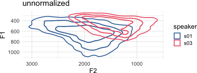
remotes::install_github("jofrhwld/tidynorm")Vowel formant frequencies are heavily influenced by vocal tract length differences between speakers. Equivalent vowels between speakers can have dramatically different frequency locations.
library(tidynorm)
library(ggplot2)options(
ggplot2.discrete.colour = c(
lapply(
1:6,
\(x) c(
"#4477AA", "#EE6677", "#228833",
"#CCBB44", "#66CCEE", "#AA3377"
)[1:x]
)
),
ggplot2.discrete.fill = c(
lapply(
1:6,
\(x) c(
"#4477AA", "#EE6677", "#228833",
"#CCBB44", "#66CCEE", "#AA3377"
)[1:x]
)
)
)
theme_set(
theme_minimal(
base_size = 16
)
)ggplot(
speaker_data,
aes(
F2, F1,
color = speaker
)
) +
ggdensity::stat_hdr(
probs = c(0.95, 0.8, 0.5),
alpha = 1,
fill = NA,
linewidth = 1
) +
scale_x_reverse() +
scale_y_reverse() +
coord_fixed() +
labs(
title = "unnormalized"
)
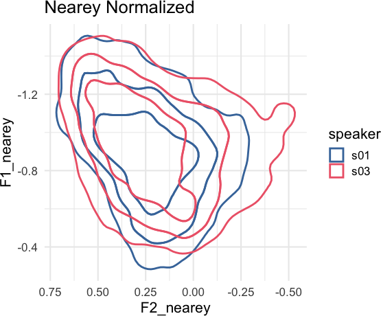
The goal of {tidynorm} is to provide tidyverse-friendly
and familiar functions that will allow you to quickly normalize vowel
formant data. There are a number of built in functions based on
conventional normalization methods.
speaker_data |>
  norm_nearey(
    F1:F3,
    .by = speaker,
    .names = "{.formant}_nearey"
  ) ->
speaker_normalized
#> Normalization info
#> • normalized with `tidynorm::norm_nearey()`
#> • normalized `F1`, `F2`, and `F3`
#> • normalized values in `F1_nearey`, `F2_nearey`, and `F3_nearey`
#> • grouped by `speaker`
#> • within formant: FALSE
#> • (.formant - mean(.formant, na.rm = T))/(1)speaker_normalized |>
ggplot(
aes(
F2_nearey, F1_nearey,
color = speaker
)
) +
ggdensity::stat_hdr(
probs = c(0.95, 0.8, 0.5),
alpha = 1,
fill = NA,
linewidth = 1
) +
scale_x_reverse() +
scale_y_reverse() +
coord_fixed() +
labs(
title = "Nearey Normalized"
)
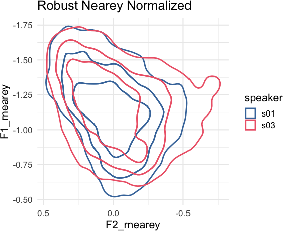
There is also a tidynorm::norm_generic() function to
allow you to define your own bespoke normalization methods. For example,
a “robust Nearey” normalization method using the median, instead of the
mean, could be done like so.
speaker_rnearey <- speaker_data |>
  norm_generic(
    F1:F3,
    .by = speaker,
    .by_formant = FALSE,
    .pre_trans = log,
    .L = median(.formant, na.rm = T),
    .names = "{.formant}_rnearey"
  )
#> Normalization info
#> • normalized with `tidynorm::norm_generic()`
#> • normalized `F1`, `F2`, and `F3`
#> • normalized values in `F1_rnearey`, `F2_rnearey`, and `F3_rnearey`
#> • grouped by `speaker`
#> • within formant: FALSE
#> • (.formant - median(.formant, na.rm = T))/(1)speaker_rnearey |>
ggplot(
aes(
F2_rnearey, F1_rnearey,
color = speaker
)
) +
ggdensity::stat_hdr(
probs = c(0.95, 0.8, 0.5),
alpha = 1,
fill = NA,
linewidth = 1
) +
scale_x_reverse() +
scale_y_reverse() +
coord_fixed() +
labs(
title = "Robust Nearey Normalized"
)