

CEC is an
R package that
performs data points clustering using the cross–entropy clustering (CEC)
method1. This method has been developed
based on information theory and combines the speed and simplicity of
k-means with the ability to use various Gaussian mixture models and
automatically remove unnecessary clusters.
CEC can
be installed directly from CRAN as follows:
install.packages("CEC")You can also use the remotes package to
install the development version of CEC as
follows:
remotes::install_github("swarm-lab/cec")The core function of the CEC package is
the cec function. In the simplest scenario, this function
requires only two arguments: an input data matrix (x) and
the initial number of cluster centers (centers). For
instance, here is how to identify two clusters in the waiting times
between eruptions for the Old Faithful geyser in Yellowstone National
Park, Wyoming, USA:
library("CEC")
data("faithful")
clusters <- cec(as.matrix(faithful[, 2, drop = FALSE]), 2)
clusters
The function cec returns the following important
information:
clusters$cluster: the cluster membership of each data
point;clusters$centers: the coordinates of the centers of
each cluster;clusters$covariances.model: the model covariance of
each cluster;clusters$probability: the probability that a random
data point belongs to a given cluster.Additional information concerning the number of iterations, the cost (energy) function, and the number of clusters at each iteration are also available.
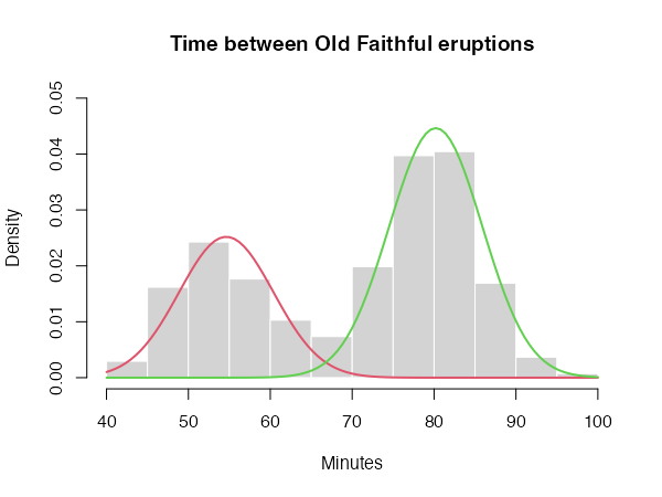
You can now plot the results of the clustering process as follows:
hist(faithful$waiting, prob = TRUE, main = "Time between Old Faithful eruptions",
     xlab = "Minutes", col = "lightgray", border = 0, ylim = c(0, 0.05))

for (i in c(1:2)) {
    curve(cec$probability[i] * dnorm(x, mean = cec$centers[i],
                                     sd = sqrt(cec$covariances.model[[i]][1])),
          add = T, col = i + 1, lwd = 2)
}
Like k-means, the quality of the results produced by CEC depends on
the choice of initial cluster centers. The initial locations of the
centers can be chosen using the centers.init parameter of
the cec function. It can be set to "random" to
select the initial centers randomly, or to "kmeans++" to
select them via the k-means++ method.
It is also recommended to run the clustering algorithm multiple times
with different cluster centers. This can easily be achieved using the
nstart parameter. For instance,
clusters <- cec(as.matrix(faithful[, 2, drop = FALSE]), 2, method = "kmeans++",
    nstart = 10, threads = 4)
clusters
will run the clustering algorithm 10 times, initializing it each time with the output of the k-means++ algorithm. Only the best of the 10 runs (i.e. the run with the lowest cost function) will be returned by the function.
Note that, when nstart > 1, the clustering process
can be sped-up by running it in parallel threads using the
threads parameter (more details in the package manual).
card.min represents the minimal cluster size, i.e. the
number of points below which a cluster is removed from the analysis. It
can be expressed as a number of points or as a percentage of the data
set size.
iter.max is the maximum allowed number of iterations of
the algorithm at each start. If the algorithm does not converge before
iter.max is reached, the function will stop and return the
best result so far.
One of the most important properties of the CEC algorithm is that it
can combined various Gaussian models in the same clustering process. The
CEC package includes six Gaussian models, which can be specified via the
parameter type. These models are:
type = "all"
The general Gaussian CEC algorithm gives similar results to those obtained by Gaussian Mixture Models. However, the CEC does not use the EM (Expectation Maximization) approach for minimization but a simple iteration process (Hartigan method). Consequently, larger data sets can be processed in shorter time.
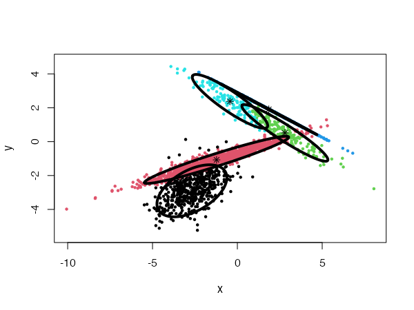
CEC will have a tendency to divide the data into clusters in the shape of ellipses (ellipsoids in higher dimensions). For instance:
data("fourGaussians")
cec <- cec(fourGaussians, centers = 10, type = "all", nstart = 20)
plot(cec, asp = 1)
type = "spherical"
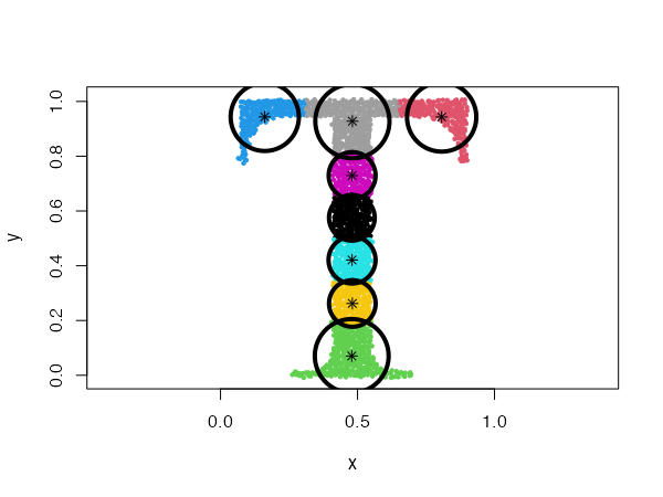
The original distribution will be approximated by spherical (radial) densities, which will result in splitting the data into disk-like clusters of arbitrary sizes (spheres in higher dimensions).
data("Tset")
cec <- cec(x = Tset, centers = 10, type = "spherical", nstart = 5)
plot(cec, asp = 1)
type = "fixedr"
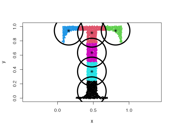
Similarly to the general spherical model, the data set will be
divided into clusters resembling disks, but with their radius determined
by the param argument.
data("Tset")
cec <- cec(x = Tset, centers = 10, type = "fixedr", param = 0.01, nstart = 20)
plot(cec, asp = 1)
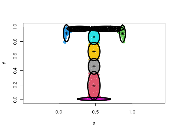
type = "diagonal"
In this case, the data will be described by ellipses for which the main semi-major axes are parallel to the axes of the coordinate system.
data("Tset")
cec <- cec(x = Tset, centers = 10, type = "diagonal", nstart = 5)
plot(cec, asp = 1)
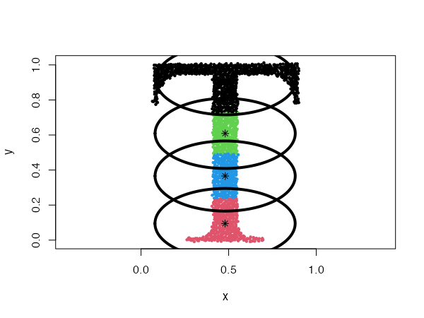
type = "covariance"
This model clusters the data using Gaussians with a fixed covariance.
The covariance matrix is passed to the param argument.
data("Tset")
cec <- cec(x = Tset, centers = 10, card.min = '10%', type = "covariance",
    param = matrix(c(0.04,  0,
                     0,     0.01), 2))
plot(cec, asp = 1)
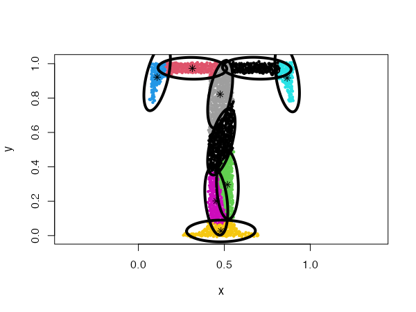
type = "eigenvalues"
This is similar to the previous example, but here the Gaussians have
fixed eigenvalues. The eigenvalues are passed to the param
argument.
data("Tset")
cec <- cec(x = Tset, centers = 10, type = "eigenvalues", param = c(0.01, 0.001),
    nstart = 5)
plot(cec, asp = 1)
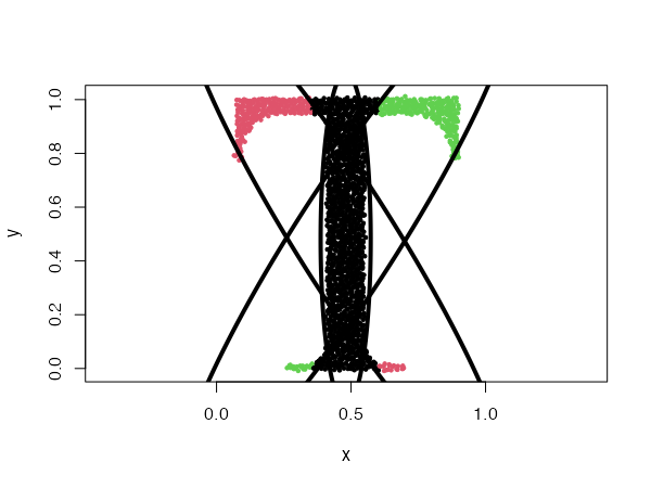
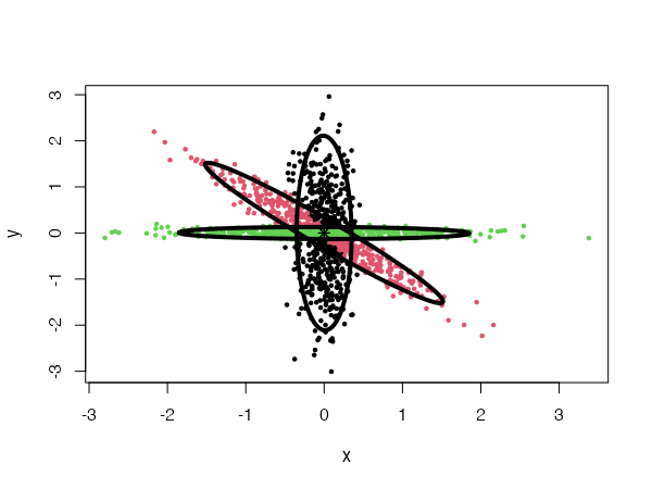
type = "mean"
In this condition, the data is clustered using Gaussians with fixed
mean values. The mean values of the data dimensions are passed to the
param argument.
data("Tset")
cec <- cec(Tset, 4, "mean", param = c(0.48, 0.48), nstart = 5)
plot(cec, asp = 1)
data("threeGaussians")
cec <- cec(threeGaussians,4, "mean", param = c(0, 0), nstart = 10)
plot(cec)
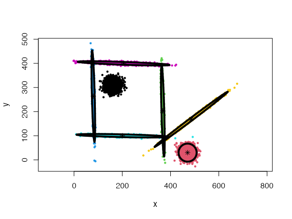
One of the most powerful properties of the CEC algorithm is the possibility of mixing Gaussian models together. More precisely, the mixed models can be specified by giving a list of cluster types (and a list of corresponding parameters, if needed).
data("mixShapes")
cec <- cec(mixShapes, 7, iter.max = 3,
    type = c("fixedr", "fixedr", "eigen", "eigen",  "eigen", "eigen", "eigen"),
    param = list(350, 350, c(9000, 8), c(9000, 8),
                 c(9000, 8), c(9000, 8), c(9000, 8)),
    nstart = 500, threads = 10)
plot(cec, asp = 1)
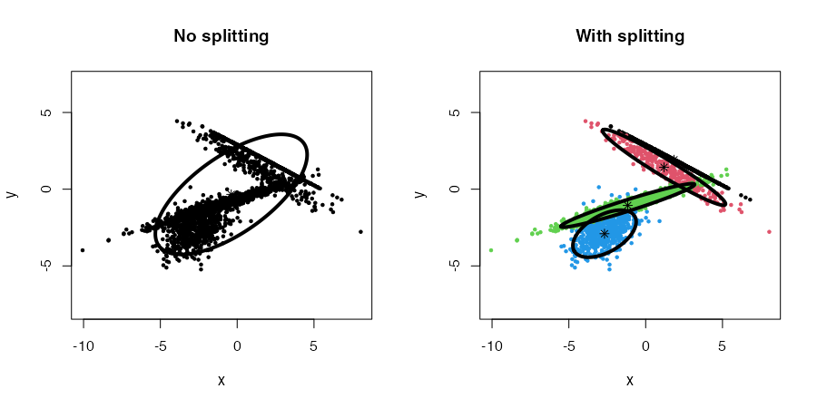
The cec function includes an option to discover new
clusters after the initial clustering has occurred. This is done by
recursively trying to split each cluster into two smaller clusters that
would lower the cost function.
To enable the splitting method, the split argument must
be set to TRUE in the cec function. For
instance:
data("fourGaussians")
par(mfrow = c(1,2))

# No splitting
cec <- cec(fourGaussians, centers = 1, type = "all")
plot(cec, asp = 1, main = "No splitting")

# With splitting
cec <- cec(fourGaussians, centers = 1, type = "all", split = TRUE)
plot(cec, asp = 1, main = "With splitting")
Combined with the nstart parameter, the whole procedure,
from start to end (initial clustering and splitting), can be repeated
multiple times. In this, case we can also use multiple threads to speed
the process up (threads parameter).
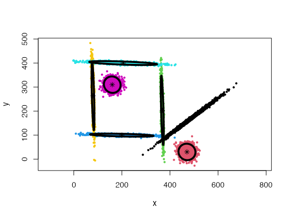
Note that the splitting method will be used implicitly when the
centers argument is not provided.
data("mixShapes")
cec <- cec(mixShapes)
plot(cec, asp = 1)
Finally, four parameters control the splitting mode:
split.depth, split.tries,
split.limit, and split.initial.starts. The
description of those parameters and their default values are provided in
the package manual. They can be useful to help the algorithm produce
meaningful clustering in more complex situations.
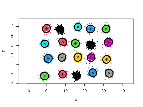
For instance, we can generate a data set of 20 Gaussians with the following code:
twenty.gaussians <- matrix(NA, 0, 2)
for (i in 0:19) {
    G <- matrix(rnorm(400), 200, 2)
    G[,1] <- G[,1] + i %% 5 * 8 + stats::runif(1,-1, 1)
    G[,2] <- G[,2] + i %/% 5 * 8 + stats::runif(1,-1, 1)
    twenty.gaussians <- rbind(twenty.gaussians, G)
}
Using a general Gaussian distributions model
(type = 'all') and no initial centers, the algorithm finds
easily the 20 Gaussian clusters, and we only need to provide it with a
low card.min value.
cec <- cec(twenty.gaussians, card.min="1%")
plot(cec, asp = 1)
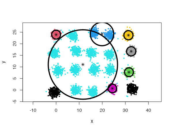
However, using spherical densities (type = 'spherical')
on the same data set will lead to sub-optimal results:
cec <- cec(twenty.gaussians, type = "spherical", card.min="1%")
plot(cec, asp = 1)
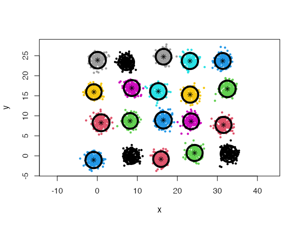
We can help the algorithm identify a more satisfying solution by
playing with the split.depth and split.tries
parameters, for instance.
cec <- cec(twenty.gaussians, type = "spherical", card.min="1%",
    split.depth = 25, split.tries = 15)
plot(cec, asp = 1)
Tabor, J., & Spurek, P. (2014). Cross-entropy clustering. Pattern Recognition, 47(9), 3046–3059. https://doi.org/10.1016/j.patcog.2014.03.006↩︎