MorphoRegions is an R package built to computationally identify regions (morphological, functional, etc.) in serially homologous structures such as, but not limited to, the vertebrate backbone. Regions are modeled as segmented linear regressions with each segment corresponding to a region and region boundaries (or breakpoints) corresponding to changes along the serially homologous structure. The optimal number of regions and their breakpoint positions are identified using maximum-likelihood methods without a priori assumptions.
This package was first presented in Gillet et al. (2024) and is an updated version of the regions R package from Jones et al. (2018) with improved computational methods and expanded fitting and plotting options.
You can install the released version of MorphoRegions from CRAN with:
install.packages("MorphoRegions")Or the development version from GitHub with:
# install.packages("remotes")
remotes::install_github("AaGillet/MorphoRegions")The following example illustrates the basic steps to prepare the
data, fit regionalization models, select the best model, and plot the
results. See vignette("MorphoRegions") or the MorphoRegions
website for a detailed guide of the package and its
functionalities.
library(MorphoRegions)Data should be provided as a dataframe where each row is an element
of the serially homologous structure (e.g., a vertebra). One column
should contain positional information of each element (e.g., vertebral
number) and other columns should contain variables that will be used to
calculate regions (e.g., morphological measurements). The
dolphin dataset contains vertebral measurements of a
dolphin with the positional information (vertebral number) in the first
column.
data("dolphin")| Vertebra | Lc | Wc | Hc | Hnp | Wnp | Inp | Ha | Wa | Lm | Wm | Hm | Hch | Wch | Ltp | Wtp | Itp | |
|---|---|---|---|---|---|---|---|---|---|---|---|---|---|---|---|---|---|
| 8 | 8 | 1.33 | 3.37 | 2.02 | 2.85 | 1.17 | 2.01 | 1.72 | 1.48 | 0.00 | 0.00 | 0.0 | 0 | 0 | 1.71 | 1.67 | 1.57 |
| 9 | 9 | 1.46 | 3.67 | 2.10 | 3.20 | 1.63 | 2.01 | 1.44 | 1.65 | 0.00 | 0.00 | 0.0 | 0 | 0 | 1.51 | 1.61 | 1.57 |
| 10 | 10 | 1.57 | 3.62 | 2.26 | 3.13 | 1.71 | 2.01 | 1.42 | 2.18 | 0.00 | 0.00 | 0.0 | 0 | 0 | 1.06 | 1.90 | 1.57 |
| 11 | 11 | 1.71 | 3.75 | 2.24 | 3.07 | 1.71 | 2.01 | 1.38 | 1.25 | 0.56 | 0.38 | 1.7 | 0 | 0 | 1.03 | 1.91 | 1.66 |
| 12 | 12 | 1.74 | 3.72 | 2.28 | 2.66 | 1.96 | 1.99 | 1.30 | 1.50 | 1.45 | 1.09 | 2.0 | 0 | 0 | 0.60 | 1.71 | 1.57 |
| 13 | 13 | 1.82 | 3.92 | 2.28 | 2.61 | 1.74 | 1.88 | 1.29 | 1.74 | 1.86 | 1.12 | 2.0 | 0 | 0 | 0.37 | 1.44 | 1.57 |
Prior to analysis, data must be processed into an object usable by
MorphoRegions using process_measurements(). The
pos argument is used to specify the name or index of the
column containing positional information and the fillNA
argument allows to fill missing values in the dataset (up to two
successive elements).
dolphin_data <- process_measurements(dolphin, pos = 1)
class(dolphin_data)
#> [1] "regions_data"
Data are then ordinated using a Principal Coordinates Analysis (PCO)
to reduce dimensionality and allow the combination of a variety of data
types. The number of PCOs to retain for analyses can be selected using
PCOselect() (see the vignette for different methods of PCO
axes selection).
dolphin_pco <- svdPCO(dolphin_data, metric = "gower")

# Select PCOs with variance > 0.05 :
PCOs <- PCOselect(dolphin_pco, method = "variance",
                  cutoff = .05)
PCOs
#> A `regions_pco_select` object
#> - PCO scores selected: 1, 2
#> - Method: variance (cutoff: 0.05)The calcregions() function allows fitting all possible
combinations of segmented linear regressions from 1 region (no
breakpoint) to the number of regions specified in the
noregions argument. In this example, up to 5 regions (4
breakpoints) will be fitted along the backbone, however, there is no
limit for this value and it is possible to fit as many regions as you
would like. For this example, regions will be fitted with a minimum of 3
vertebrae per region (minvert = 3) and using a continuous
fit (cont = TRUE) (see
vignette("MorphoRegions") or MorphoRegions
website for details about fitting options).
regionresults <- calcregions(dolphin_pco, scores = PCOs, noregions = 5,
                             minvert = 3, cont = TRUE,
                             exhaus = TRUE, verbose = FALSE)
regionresults
#> A `regions_results` object
#>  - number of PCOs used: 2
#>  - number of regions: 1, 2, 3, 4, 5
#>  - model type: continuous
#>  - min vertebrae per region: 3
#>  - total models saved: 28810
#> Use `summary()` to examine summaries of the fitting process.
For each given number of regions, the best fit is selected by
minimizing the residual sum of squares (sumRSS):
models <- modelselect(regionresults)
models
#>  Regions BP 1 BP 2 BP 3 BP 4 sumRSS RSS.1 RSS.2
#>        1    .    .    .    .  1.898 1.456 0.441
#>        2   26    .    .    .  0.413 0.105 0.308
#>        3   23   29    .    .  0.147 0.092 0.055
#>        4   23   30   40    .  0.073 0.034 0.040
#>        5   23   27   34   40  0.046 0.026 0.020
The best overall model (best number of regions) is then select by ordering models from the best fit (top row) to the worst fit (last row) using either the AICc or BIC criterion:
supp <- modelsupport(models)
supp
#> - Model support (AICc)
#>  Regions BP 1 BP 2 BP 3 BP 4 sumRSS     AICc deltaAIC model_lik Ak_weight
#>        5   23   27   34   40  0.046 -556.036    0.000         1         1
#>        4   23   30   40    .  0.073 -528.096   27.940         0         0
#>        3   23   29    .    .  0.147 -480.952   75.084         0         0
#>        2   26    .    .    .  0.413 -405.787  150.250         0         0
#>        1    .    .    .    .  1.898 -290.769  265.267         0         0
#> Region score: 5
#>
#> - Model support (BIC)
#>  Regions BP 1 BP 2 BP 3 BP 4 sumRSS      BIC deltaBIC model_lik BIC_weight
#>        5   23   27   34   40  0.046 -526.559    0.000         1          1
#>        4   23   30   40    .  0.073 -502.645   23.914         0          0
#>        3   23   29    .    .  0.147 -460.321   66.238         0          0
#>        2   26    .    .    .  0.413 -390.668  135.891         0          0
#>        1    .    .    .    .  1.898 -281.774  244.784         0          0
#> Region score: 5
Here, for both criteria, the best model is the 5 regions models with
breakpoints at vertebrae 23, 27, 34, and 40. The breakpoint value
corresponds to the last vertebra included in the region, so the first
region here is made of vertebrae 8 to 23 included and the second region
is made of vertebrae 24 to 27. The function also returns the
region score, a continuous value reflecting the level
of regionalization while accounting for uncertainty in the best number
of regions (see vignette("MorphoRegions") or MorphoRegions
website for more details).
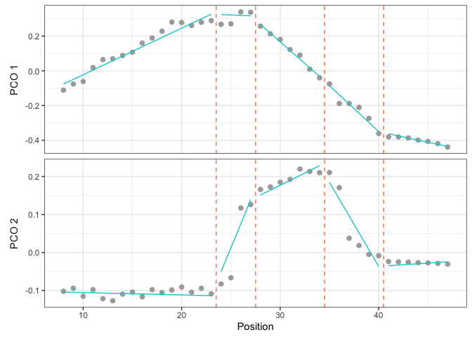
Results of the best model (or any other model) can be visualized either as a scatter plot or as a vertebral map.
The scatter plot shows the PCO score (here for PCO 1 and 2) of each vertebra along the backbone (gray dots) and the segmented linear regressions (cyan line) of the model to plot. Breakpoints are showed by dotted orange lines.
plotsegreg(dolphin_pco, scores = 1:2, modelsupport = supp,
           criterion = "bic", model = 1)
In the vertebral map plot, each vertebra is
represented by a rectangle color-coded according to the region to which
it belongs. Vertebrae not included in the analysis (here vertebrae 1 to
7) are represented by gray rectangles and can be removed using
dropNA = TRUE.
plotvertmap(dolphin_pco, name = "Dolphin", modelsupport = supp,
            criterion = "bic", model = 1)

plotvertmap(dolphin_pco, name = "Dolphin", modelsupport = supp,
            criterion = "bic", model = 1, dropNA = TRUE)

The variability around breakpoint positions can be calculated using
calcBPvar() and then displayed on the vertebral map. The
weighted average position of each breakpoint is shown by the black dot
and the weighted variance is illustrated by the horizontal black
bar.
bpvar <- calcBPvar(regionresults, noregions = 5,
                   pct = 0.1, criterion = "bic")

plotvertmap(dolphin_pco, name = "Dolphin",
            dropNA = TRUE, bpvar = bpvar)
To cite MorphoRegions, please use:
citation("MorphoRegions")