The itp package implements the Interpolate, Truncate, Project (ITP) root-finding algorithm of Oliveira and Takahashi (2021). Each iteration of the algorithm results in a bracketing interval for the root that is narrower than the previous interval. It’s performance compares favourably with existing methods on both well-behaved functions and ill-behaved functions while retaining the worst-case reliability of the bisection method. For details see the authors’ Kudos summary and the Wikipedia article ITP method.
We use three examples from Section 3 of Oliveira and Takahashi (2021)
to illustrate the use of the itp function. Each of these
functions has a root in the interval \((-1,
1)\). The function can be supplied either as an R function or as
an external pointer to a C++ function.
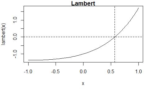
library(itp)The Lambert function \(l(x) = xe^x - 1\) is continuous.

The itp function finds an estimate of the root, that is,
\(x^{\ast}\) for which \(f(x^{\ast})\) is (approximately) equal to
0. The algorithm continues until the length of the interval that
brackets the root is smaller than \(2
\epsilon\), where \(\epsilon\)
is a user-supplied tolerance. The default is \(\epsilon = 10^{-10}\).
First, we supply an R function that evaluates the Lambert function.
# Lambert, using an R function
lambert <- function(x) x * exp(x) - 1
itp(lambert, c(-1, 1))
#> function: lambert
#>       root     f(root)  iterations
#>     0.5671   2.048e-12           8
Now, we create an external pointer to a C++ function that has been
provided in the itp package and pass this pointer to the
function itp(). For more information see the Overview
of the itp package vignette.
# Lambert, using an external pointer to a C++ function
lambert_ptr <- xptr_create("lambert")
itp(lambert_ptr, c(-1, 1))
#> function: lambert_ptr
#>       root     f(root)  iterations
#> 0.5671 2.048e-12 8itp_cAlso provided is the function itp_c, which is equivalent
to itp, but the calculations are performed entirely using
C++, and the arguments differ slightly: itp_c has a named
required argument pars rather than ... and it
does not have the arguments interval, f.a or
f.b.
# Calling itp_c()
res <- itp_c(lambert_ptr, pars = list(), a = -1, b = 1)
res
#> function:
#>       root     f(root)  iterations
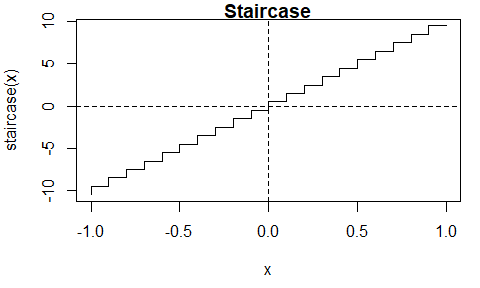
#> 0.5671 2.048e-12 8The staircase function \(s(x) = \lceil 10 x - 1 \rceil + 1/2\) is discontinuous.

The itp function finds the discontinuity at \(x = 0\) at which the sign of the function
changes. The value of 0.5 returned for the root res$root is
the midpoint of the bracketing interval [res$a, res$b] at
convergence.
# Staircase
staircase <- function(x) ceiling(10 * x - 1) + 1 / 2
res <- itp(staircase, c(-1, 1))
print(res, all = TRUE)
#> function: staircase
#>       root     f(root)  iterations           a           b         f.a
#>  7.404e-11         0.5          31           0   1.481e-10        -0.5
#>        f.b   precision
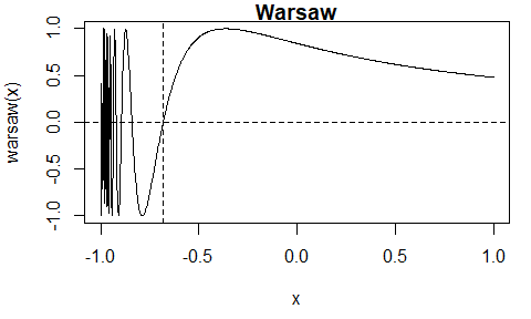
#> 0.5 7.404e-11The Warsaw function \(w(x) = I(x > -1)\left(1 + \sin\left(\frac{1}{1+x}\right)\right)-1\) has multiple roots.

When the initial interval is \([-1,
1]\) the itp function finds the root \(x \approx -0.6817\). There are other roots
that could be found from a different initial interval.
# Warsaw
warsaw <- function(x) ifelse(x > -1, sin(1 / (x + 1)), -1)
itp(warsaw, c(-1, 1))
#> function: warsaw
#>       root     f(root)  iterations
#> -0.6817 -5.472e-11 11To get the current released version from CRAN:
install.packages("itp")See the Overview
of the itp package vignette, which can also be accessed using
vignette("itp-vignette", package = "itp").