Robust and reproducible non-linear regression in R
Daniel Padfield: d.padfield@exeter.ac.uk
Granville Matheson: mathesong@gmail.com
Francis Windram: francis.windram17@imperial.ac.uk
Please report any issues/suggestions for improvement in the issues link for the repository. Or please email d.padfield@exeter.ac.uk or mathesong@gmail.com.
This package is licensed under GPL-3.
nls.multstart is an R package that allows more robust and reproducible non-linear regression compared to nls() or nlsLM(). These functions allow only a single starting value, meaning that it can be hard to get the best estimated model. This is especially true if the same model is fitted over many levels of a factor, which may have the same shape of curve, but be very different in terms of parameter estimates.
nls_multstart() is the main (currently only) function of nls.multstart. Similar to the R package nls2, it allows multiple starting values for each parameter and then iterates through multiple starting values, attempting a fit with each set of start parameters. The best model is then picked on AIC score. This results in a more reproducible and reliable method of fitting non-linear least squares regression in R.
This package is designed to work with the tidyverse, harnessing the functions within broom, tidyr, dplyr and purrr to extract estimates and plot things easily with ggplot2.
nls.multstart can be installed from CRAN using install.packages() or from GitHub using remotes.
# install package
install.packages('nls.multstart') # from CRAN
remotes::install_github("padpadpadpad/nls.multstart") # from GitHubnls_multstart() can be used to do non-linear regression on a single curve.
# load in nls.multstart and other packages
library(nls.multstart)
library(ggplot2)
library(broom)
library(purrr)
library(dplyr)
library(tidyr)
library(nlstools)

# load in example data set
data("Chlorella_TRC")

# define the Sharpe-Schoolfield equation
schoolfield_high <- function(lnc, E, Eh, Th, temp, Tc) {
  Tc <- 273.15 + Tc
  k <- 8.62e-5
  boltzmann.term <- lnc + log(exp(E/k*(1/Tc - 1/temp)))
  inactivation.term <- log(1/(1 + exp(Eh/k*(1/Th - 1/temp))))
  return(boltzmann.term + inactivation.term)
  }
# subset dataset
d_1 <- subset(Chlorella_TRC, curve_id == 1)
# run nls_multstart with shotgun approach
fit <- nls_multstart(ln.rate ~ schoolfield_high(lnc, E, Eh, Th, temp = K, Tc = 20),
data = d_1,
iter = 250,
start_lower = c(lnc=-10, E=0.1, Eh=0.5, Th=285),
start_upper = c(lnc=10, E=2, Eh=5, Th=330),
supp_errors = 'Y',
convergence_count = 100,
na.action = na.omit,
lower = c(lnc = -10, E = 0, Eh = 0, Th = 0))
fit
#> Nonlinear regression model
#> model: ln.rate ~ schoolfield_high(lnc, E, Eh, Th, temp = K, Tc = 20)
#> data: data
#> lnc E Eh Th
#> -1.3462 0.9877 4.3326 312.1887
#> residual sum-of-squares: 7.257
#>
#> Number of iterations to convergence: 14
#> Achieved convergence tolerance: 1.49e-08This method uses a random-search/shotgun approach to
fit multiple curves. Random start parameter values are picked from a
uniform distribution between start_lower() and
start_upper() for each parameter. If the best model is not
improved upon (in terms of AIC score) for 100 new start parameter
combinations, the function will return that model fit. This is
controlled by convergence_count, if this is set to
FALSE, nls_multstart() will try and fit
all iterations.
An alternative to the shotgun approach is to use Latin
Hypercube Sampling (LHS), which can only be used when
iter is set to a single number. Instead of sampling from a
uniform distribution across the bounds of each parameter, these methods
try to take a set of samples from the range of parameter values that
covers the parameter space optimally for any given set of parameters.
This approach can result in less iterations being needed to get the
same reliability of model fitting than either the shotgun or grid-start
approaches. You can specify different methods used for the LHS
using lhstype. Options are “random”, “improved”, maximin”,
or “genetic”. You can learn more about the options on the lhs package
website.
# subset dataset
d_1 <- subset(Chlorella_TRC, curve_id == 1)

# run nls_multstart with shotgun approach
fit <- nls_multstart(ln.rate ~ schoolfield_high(lnc, E, Eh, Th, temp = K, Tc = 20),
                     data = d_1,
                     iter = 250,
                     start_lower = c(lnc=-10, E=0.1, Eh=0.5, Th=285),
                     start_upper = c(lnc=10, E=2, Eh=5, Th=330),
                     supp_errors = 'Y',
                     convergence_count = 100,
                     na.action = na.omit,
                     lower = c(lnc = -10, E = 0, Eh = 0, Th = 0),
                     lhstype = 'improved')

fit
#> Nonlinear regression model
#>   model: ln.rate ~ schoolfield_high(lnc, E, Eh, Th, temp = K, Tc = 20)
#>    data: data
#>      lnc        E       Eh       Th
#>  -1.3462   0.9877   4.3326 312.1887
#>  residual sum-of-squares: 7.257
#>
#> Number of iterations to convergence: 11
#> Achieved convergence tolerance: 1.49e-08
Another method of model fitting available in
nls_multstart() is a gridstart approach. This method
creates a combination of start parameters, equally spaced across each of
the starting parameter bounds. This can be specified with a vector of
the same length as the number of parameters, c(5, 5, 5) for
3 estimated parameters will yield 125 iterations.
# run nls_multstart with gridstart approach
fit <- nls_multstart(ln.rate ~ schoolfield_high(lnc, E, Eh, Th, temp = K, Tc = 20),
                     data = d_1,
                     iter = c(5, 5, 5, 5),
                     start_lower = c(lnc=-10, E=0.1, Eh=0.5, Th=285),
                     start_upper = c(lnc=10, E=2, Eh=5, Th=330),
                     supp_errors = 'Y',
                     na.action = na.omit,
                     lower = c(lnc = -10, E = 0, Eh = 0, Th = 0))

fit
#> Nonlinear regression model
#>   model: ln.rate ~ schoolfield_high(lnc, E, Eh, Th, temp = K, Tc = 20)
#>    data: data
#>      lnc        E       Eh       Th
#>  -1.3462   0.9877   4.3326 312.1887
#>  residual sum-of-squares: 7.257
#>
#> Number of iterations to convergence: 17
#> Achieved convergence tolerance: 1.49e-08
Reassuringly all methods give identical model fits!
This fit can then be tidied up in various ways using the R package broom. Each different function in broom returns a different set of information. tidy() returns the estimated parameters, augment() returns the predictions and glance() returns information about the model such as AIC score. Confidence intervals of non-linear regression can also be estimated using nlstools::confint2()
# get info
info <- glance(fit)
info
#> # A tibble: 1 × 9
#>   sigma isConv       finTol logLik   AIC   BIC deviance df.residual  nobs
#>   <dbl> <lgl>         <dbl>  <dbl> <dbl> <dbl>    <dbl>       <int> <int>
#> 1 0.952 TRUE   0.0000000149  -14.0  38.0  40.4     7.26           8    12

# get params
params <- tidy(fit)

# get confidence intervals using nlstools
CI <- confint2(fit) %>%
  data.frame() %>%
  rename(., conf.low = X2.5.., conf.high = X97.5..)

# bind params and confidence intervals
params <- bind_cols(params, CI)
select(params, -c(statistic, p.value))
#> # A tibble: 4 × 5
#>   term  estimate std.error conf.low conf.high
#>   <chr>    <dbl>     <dbl>    <dbl>     <dbl>
#> 1 lnc     -1.35      0.466  -2.42      -0.272
#> 2 E        0.988     0.452  -0.0549     2.03
#> 3 Eh       4.33      1.49    0.902      7.76
#> 4 Th     312.        3.88  303.       321.

# get predictions
preds <- augment(fit)
preds
#> # A tibble: 12 × 5
#>    ln.rate     K `(weights)` .fitted  .resid
#>      <dbl> <dbl>       <dbl>   <dbl>   <dbl>
#>  1 -2.06    289.           1 -1.89   -0.176
#>  2 -1.32    292.           1 -1.48    0.156
#>  3 -0.954   295.           1 -1.08    0.127
#>  4 -0.794   298.           1 -0.691  -0.103
#>  5 -0.182   301.           1 -0.311   0.129
#>  6  0.174   304.           1  0.0534  0.121
#>  7 -0.0446  307.           1  0.367  -0.411
#>  8  0.481   310.           1  0.498  -0.0179
#>  9  0.388   313.           1  0.180   0.208
#> 10  0.394   316.           1 -0.645   1.04
#> 11 -3.86    319.           1 -1.70   -2.16
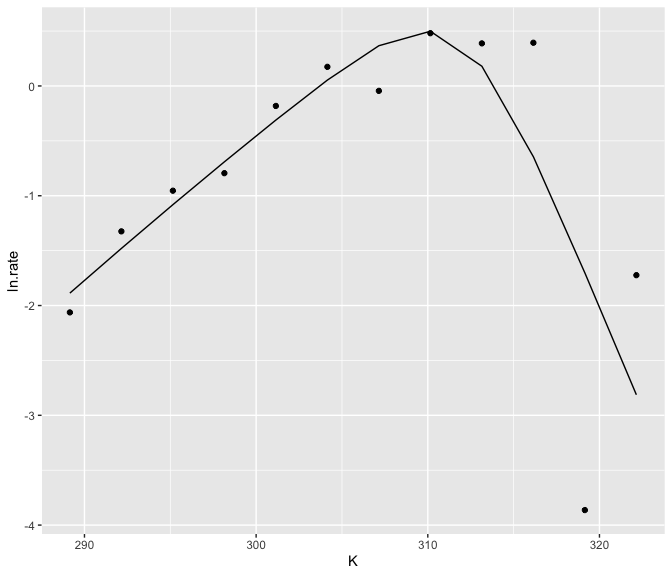
#> 12 -1.72 322. 1 -2.81 1.09The predictions can then easily be plotted alongside the actual data.
ggplot() +
  geom_point(aes(K, ln.rate), d_1) +
  geom_line(aes(K, .fitted), preds)
nls_multstart() is unlikely to speed you up very much if only one curve is fitted. However, if you have 10, 60 or 100s of curves to fit, it makes sense that at least some of them may not fit with the same starting parameters, no matter how many iterations it is run for.
This is where nls_multstart() can help. Multiple models can be fitted using purrr, dplyr and tidyr. These fits can then be tidied using broom, an approach Hadley Wickham has previously written about.
# fit over each set of groupings
fits <- Chlorella_TRC %>%
  group_by(., flux, growth.temp, process, curve_id) %>%
  nest() %>%
  mutate(fit = purrr::map(data, ~ nls_multstart(ln.rate ~ schoolfield_high(lnc, E, Eh, Th, temp = K, Tc = 20),
                                   data = .x,
                                   iter = 1000,
                                   start_lower = c(lnc=-1000, E=0.1, Eh=0.5, Th=285),
                                   start_upper = c(lnc=1000, E=2, Eh=10, Th=330),
                                   supp_errors = 'Y',
                                   na.action = na.omit,
                                   lower = c(lnc = -10, E = 0, Eh = 0, Th = 0))))
A single fit can check to make sure it looks ok. Looking at
fits demonstrates that there is now a fit list
column containing each of the non-linear fits for each combination of
our grouping variables.
# look at output object
select(fits, curve_id, data, fit)
#> Adding missing grouping variables: `flux`, `growth.temp`, `process`
#> # A tibble: 60 × 6
#> # Groups:   flux, growth.temp, process, curve_id [60]
#>    flux        growth.temp process     curve_id data              fit
#>    <chr>             <dbl> <chr>          <dbl> <list>            <list>
#>  1 respiration          20 acclimation        1 <tibble [12 × 3]> <nls>
#>  2 respiration          20 acclimation        2 <tibble [12 × 3]> <nls>
#>  3 respiration          23 acclimation        3 <tibble [12 × 3]> <nls>
#>  4 respiration          27 acclimation        4 <tibble [9 × 3]>  <nls>
#>  5 respiration          27 acclimation        5 <tibble [12 × 3]> <nls>
#>  6 respiration          30 acclimation        6 <tibble [12 × 3]> <nls>
#>  7 respiration          30 acclimation        7 <tibble [12 × 3]> <nls>
#>  8 respiration          33 acclimation        8 <tibble [10 × 3]> <nls>
#>  9 respiration          33 acclimation        9 <tibble [8 × 3]>  <nls>
#> 10 respiration          20 acclimation       10 <tibble [10 × 3]> <nls>
#> # ℹ 50 more rows

# look at a single fit
summary(fits$fit[[1]])
#>
#> Formula: ln.rate ~ schoolfield_high(lnc, E, Eh, Th, temp = K, Tc = 20)
#>
#> Parameters:
#>     Estimate Std. Error t value Pr(>|t|)
#> lnc  -1.3462     0.4656  -2.891   0.0202 *
#> E     0.9877     0.4521   2.185   0.0604 .
#> Eh    4.3326     1.4878   2.912   0.0195 *
#> Th  312.1887     3.8782  80.499 6.32e-13 ***
#> ---
#> Signif. codes:  0 '***' 0.001 '**' 0.01 '*' 0.05 '.' 0.1 ' ' 1
#>
#> Residual standard error: 0.9524 on 8 degrees of freedom
#>
#> Number of iterations to convergence: 15
#> Achieved convergence tolerance: 1.49e-08These fits can be cleaned up in a similar way to the single fit, but this time purrr::map() iterates the broom function over the grouping variables.
# get summary
info <- fits %>%
  mutate(summary = map(fit, glance)) %>%
  unnest(summary)

# get params
params <- fits %>%
  mutate(., p = map(fit, tidy)) %>%
  unnest(p)

# get confidence intervals
CI <- fits %>%
  mutate(., cis = map(fit, confint2),
         cis = map(cis, data.frame)) %>%
  unnest(cis) %>%
  rename(., conf.low = X2.5.., conf.high = X97.5..) %>%
  group_by(., curve_id) %>%
  mutate(., term = c('lnc', 'E', 'Eh', 'Th')) %>%
  ungroup() %>%
  select(., -data, -fit)

# merge parameters and CI estimates
params <- merge(params, CI, by = intersect(names(params), names(CI)))

# get predictions
preds <- fits %>%
  mutate(., p = map(fit, augment)) %>%
  unnest(p)
Looking at info allows us to see if all the models converged.
select(info, curve_id, logLik, AIC, BIC, deviance, df.residual)
#> Adding missing grouping variables: `flux`, `growth.temp`, `process`
#> # A tibble: 60 × 9
#> # Groups:   flux, growth.temp, process, curve_id [60]
#>    flux    growth.temp process curve_id  logLik   AIC   BIC deviance df.residual
#>    <chr>         <dbl> <chr>      <dbl>   <dbl> <dbl> <dbl>    <dbl>       <int>
#>  1 respir…          20 acclim…        1 -14.0   38.0  40.4     7.26            8
#>  2 respir…          20 acclim…        2  -1.20  12.4  14.8     0.858           8
#>  3 respir…          23 acclim…        3  -7.39  24.8  27.2     2.41            8
#>  4 respir…          27 acclim…        4  -0.523 11.0  12.0     0.592           5
#>  5 respir…          27 acclim…        5 -10.8   31.7  34.1     4.29            8
#>  6 respir…          30 acclim…        6  -8.52  27.0  29.5     2.91            8
#>  7 respir…          30 acclim…        7  -1.29  12.6  15.0     0.871           8
#>  8 respir…          33 acclim…        8 -13.4   36.7  38.2     8.48            6
#>  9 respir…          33 acclim…        9   1.82   6.36  6.76    0.297           4
#> 10 respir…          20 acclim…       10  -1.27  12.5  14.1     0.755           6
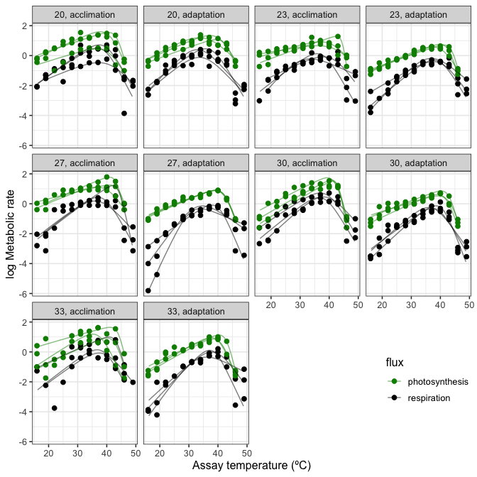
#> # ℹ 50 more rowsWhen plotting non-linear fits, it often looks better to have a smooth
curve, even if there are not many points underlying the fit. This can be
achieved by including newdata in the
augment() function and creating a higher resolution set
of predictor values.
However, when predicting for many different fits, it is not certain that each curve has the same range of predictor variables. Consequently, we need to filter each new prediction by the min() and max() of the predictor variables.
# new data frame of predictions
new_preds <- Chlorella_TRC %>%
  do(., data.frame(K = seq(min(.$K), max(.$K), length.out = 150), stringsAsFactors = FALSE))

# max and min for each curve
max_min <- group_by(Chlorella_TRC, curve_id) %>%
  summarise(., min_K = min(K), max_K = max(K)) %>%
  ungroup()

# create new predictions
preds2 <- fits %>%
  mutate(., p = map(fit, augment, newdata = new_preds)) %>%
  unnest(p) %>%
  merge(., max_min, by = 'curve_id') %>%
  group_by(., curve_id) %>%
  filter(., K > unique(min_K) & K < unique(max_K)) %>%
  rename(., ln.rate = .fitted) %>%
  ungroup()
These can then be plotted using ggplot2.
# plot
ggplot() +
  geom_point(aes(K - 273.15, ln.rate, col = flux), size = 2, Chlorella_TRC) +
  geom_line(aes(K - 273.15, ln.rate, col = flux, group = curve_id), alpha = 0.5, preds2) +
  facet_wrap(~ growth.temp + process, labeller = labeller(.multi_line = FALSE)) +
  scale_colour_manual(values = c('green4', 'black')) +
  theme_bw(base_size = 12) +
  ylab('log Metabolic rate') +
  xlab('Assay temperature (ºC)') +
  theme(legend.position = c(0.9, 0.15))
#> Warning: A numeric `legend.position` argument in `theme()` was deprecated in ggplot2
#> 3.5.0.
#> ℹ Please use the `legend.position.inside` argument of `theme()` instead.
#> This warning is displayed once every 8 hours.
#> Call `lifecycle::last_lifecycle_warnings()` to see where this warning was
#> generated.
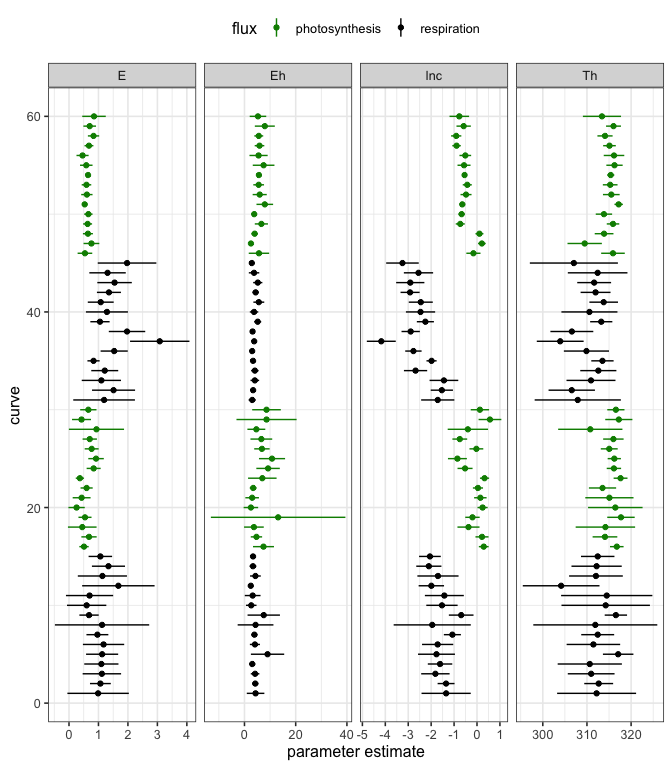
The confidence intervals of each parameter for each curve fit can also be easily visualised.
# plot
ggplot(params, aes(col = flux)) +
  geom_point(aes(curve_id, estimate)) +
  facet_wrap(~ term, scale = 'free_x', ncol = 4) +
  geom_linerange(aes(curve_id, ymin = conf.low, ymax = conf.high)) +
  coord_flip() +
  scale_color_manual(values = c('green4', 'black')) +
  theme_bw(base_size = 12) +
  theme(legend.position = 'top') +
  xlab('curve') +
  ylab('parameter estimate')