tableMatrix package provides two classes extending data.table class.
Simple tableList class wraps data.table and any additional
structures together. More complex tableMatrix class
combines data.table and matrix.
From CRAN:
install.packages("tableMatrix")From github:
# install.packages("devtools")
devtools::install_github("InferenceTechnologies/tableMatrix")Goal is to wrap data.table class and other structures together and preserve data.table behaviour.
Combine data and linear model into one object.
data(chickwts)

# Bundle chickwts data.frame together with a linear model
TL <- tableList(chickwts, lm(weight~feed, chickwts))

# tableList behaves like a data.table
mean(TL[feed=="casein", weight])
#> [1] 323.5833

# Aid part of the tableList object carries the linear model
aid(TL)
#>
#> Call:
#> lm(formula = weight ~ feed, data = chickwts)
#>
#> Coefficients:
#>   (Intercept)  feedhorsebean    feedlinseed   feedmeatmeal    feedsoybean
#>       323.583       -163.383       -104.833        -46.674        -77.155
#> feedsunflower
#> 5.333Let’s have a dataset with the following structure: first set of
columns of varying types is intented as meta data, second set of columns
of the same type is intended as main data. tableMatrix
stores meta data as a data.table and main data as a matrix. It also
keeps track of dimensions of main data, thus allowing to combine rows of
varying lengths into one object. As in tableList, tableMatrix can carry
any additional aid data.
Working with bitmaps of different sizes. Datasets
images8By8 and images10By10 contain 8x8 and
10x10 images in the form of vectors. For each row first three columns
represent image meta data, remaining columns represent the image itself.
For more information see ?images8By8.
# Load datasets
data(images8By8)
data(images10By10)

# Create a signle tableMatrix object from both datasets
# First 3 columns used as meta data, the rest as main data with corresponding dimensions
TM <- tableMatrix(list(images8By8, images10By10),
list(1:3, 1:3), list(c(4:ncol(images8By8)),c(4:ncol(images10By10))), list(c(8,8), c(10,10)))

# Default print displays the table (meta data) part
TM
#>      direction dimX dimY
#>   1:      down    8    8
#>   2:      down    8    8
#>   3:      down    8    8
#>   4:      down    8    8
#>   5:      down    8    8
#>  ---
#> 176:      both   10   10
#> 177:      both   10   10
#> 178:      both   10   10
#> 179:      both   10   10
#> 180:      both   10   10

# Number of matrices stored in the matrix (main data) part
length(mat(TM))
#> [1] 2

# Dimensions of the matrix part
matDim(TM)
#>    tm.matN tm.matDim1 tm.matDim2
#> 1:       1          8          8
#> 2:       2         10         10

# Aid part is empty
aid(TM)
#> list()


# Image data for first row
img <- getRow(TM, 1)

# Restoring dimensions of the image
dim(img) <- getRowDim(TM, 1)

# Visualising the image
image(img, axes=F)
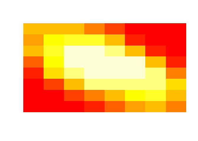
Let’s create a heat map
# Subsetting via bracket passed to the table (meta data) part
# We choose first matrix type, down direction
TM1down <- TM[.(1)][direction=="down"]

# One matrix in the matrix part of TM1down
length(mat(TM1down))
#> [1] 1

# One dimension row
matDim(TM1down)
#>    tm.matN tm.matDim1 tm.matDim2
#> 1:       1          8          8

# Heatmap
imgHeat <- colMeans(mat(TM1down, 1))

# Restoring dimensions of the heatmap
dim(imgHeat) <- getRowDim(TM1down, 1)

# Visualising heatmap
image(imgHeat, axes=F)